Figure 7.1: Matrix
In this chapter, we will introduce learning of singular value decomposition and applications using singular value decomposition from the basics and applications of linear algebra. Although I learned linear algebra in high school students and university students, I think that there are many people who do not know how it is used, so I wrote this time. In this chapter, in order to prioritize ease of understanding , explanations are given in two dimensions and within the range of real numbers. Therefore, there are some differences from the actual definition of linear algebra, but we would appreciate it if you could read it as appropriate.
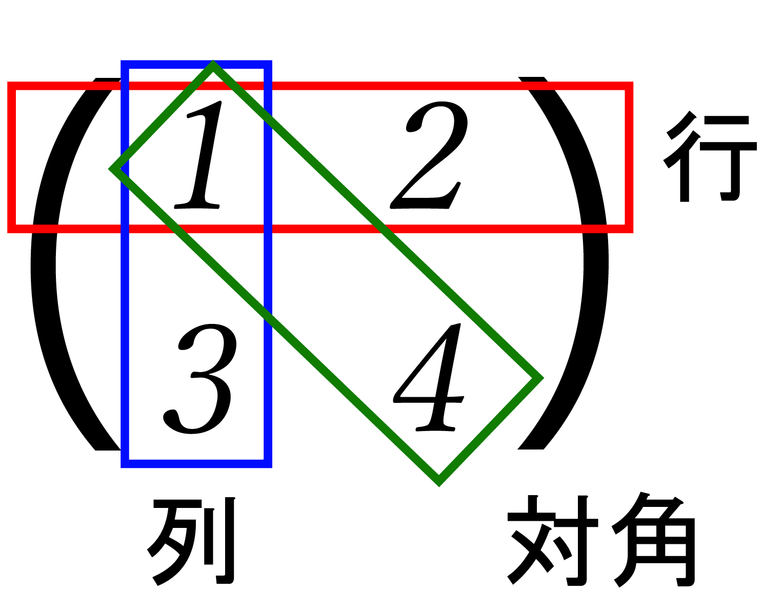
Most readers may have heard the word matrix once (currently, they don't learn matrices in high school ...). Matrix is a number like this: Refers to those arranged vertically and horizontally.
The horizontal direction is the row , the vertical direction is the column , the diagonal direction is the diagonal , and each number is called a matrix element .
Figure 7.1: Matrix
By the way, the matrix is called Matrix in English.
Let's take a quick look at the basics of matrix operations. If you are already familiar with it, you can skip this section.
Similar to the four arithmetic operations of scalars, there are additions, subtractions, multiplications and divisions in matrices. For simplicity, quadratic square matrices * 1 \ mbox {\ boldmath $ A $} and \ mbox {\ boldmath $ B $} , The 2D vector \ mbox {\ boldmath $ c $} is defined below.
[* 1] Square matrix \ cdots A matrix with the same number of rows and columns.
Matrix addition calculates the sum for each element, as in the formula (\ ref {plus}).
Matrix subtraction calculates the difference element by element, as in the formula (\ ref {minus}).
Matrix multiplication is a bit more complicated, like an expression (\ ref {times}).
Please note that if you reverse the order of multiplication, the calculation result will also change.
Matrix division uses a concept called the inverse matrix , which is a little different from division in scalars . First of all, scalars have the property that when multiplied by their own reciprocal, they always become 1.
In other words, the act of division is equivalent to the operation of "multiplying the reciprocal".
Replacing this with a matrix, we can say that what produces the identity matrix over the matrix is the matrix that represents division. In the matrix, the one corresponding to 1 in the scalar is called the identity matrix and is defined below. ..
As with the scalar 1 , the value does not change when the identity matrix is applied to any matrix.
With these in mind, let's consider matrix division. If the inverse matrix is \ mbox {\ boldmath $ M $} ^ {-1} , the definition of the inverse matrix is as follows.
Derivation is omitted, but the elements of the inverse matrix of the matrix \ mbox {\ boldmath $ A $} are defined below.
At this time, a_ {00} a_ {11} --a_ {01} a_ {10} is called a determinant (Determinant) and is expressed as det (\ mbox {\ boldmath $ A $}) .
A matrix can transform the coordinates pointed to by a vector by multiplying it by a vector. As you know, in CG, it is mostly used as a coordinate transformation matrix (world, projection, view transformation matrix). The product of and the vector is defined below.
From this section, I will explain the concept of the matrix in the range learned at the university. I think that there are many parts that seem a little difficult, but to understand Shape Matching, this concept is necessary, so do your best. However, since the story in this section is also absorbed inside the matrix operation library, there is no problem in implementing it even if you skip to section \ ref {shape matching}.
The transposed matrix is the swapped rows and columns of the elements and is defined below.
A matrix that satisfies \ mbox {\ boldmath $ A $} ^ {T} = \ mbox {\ boldmath $ A $} is called a symmetric matrix.
Given the square matrix \ mbox {\ boldmath $ A $} ,
Meet the \ lambda a, \ Mbox {\ Boldmath $ A $} of eigenvalues , \ Mbox {\ Boldmath $ V $} the eigenvectors is called.
The calculation method of eigenvalues and eigenvectors is shown below. First, the formula (\ ref {eigen}) is transformed.
Here, using the condition \ mbox {\ boldmath $ v $} \ neq 0 , the expression (\ ref {eigen2}) becomes:
Becomes. Expanding this expression, \ lambda to become a quadratic equation for, by solving this \ lambda can be calculated. Moreover, each of the calculated \ lambda expressions (\ ref { By substituting into eigen2}), you can calculate the eigenvector \ mbox {\ boldmath $ v $} .
Since the concept of eigenvalues and eigenvectors is difficult to understand from mathematical formulas alone, I think you should also read the Qiita article (described at the end of the chapter) where eigenvalues were visualized by @ kenmatsu4.
The eigenvalues and eigenvectors in the square matrix \ mbox {\ boldmath $ A $} can be used to represent the matrix \ mbox {\ boldmath $ A $} in different ways. First, the eigenvalues \ lambda are sorted by size . , Create a matrix \ mbox {\ boldmath $ \ Lambda $} with it as a diagonal element . Next, a matrix \ mbox {\ boldmath $ V $} in which the eigenvectors corresponding to each eigenvalue are arranged in order from the left . Then, the expression ( \ ref {eigen} ) can be rewritten using these matrices as follows.
Furthermore, multiply this by \ mbox {\ boldmath $ V $} ^ {-1} from the right of both sides so that the matrix \ mbox {\ boldmath $ A $} remains on the left side .
Will be.
Decomposing a matrix into a form like an expression (\ ref {eigendecomp}) in this way is called eigenvalue decomposition of a matrix.
A set of vectors that are perpendicular to each other and each is a unit vector is called an orthonormal basis. Any vector can be represented using a set of orthonormal bases * 2. In the case of two dimensions, There are two vectors that can be orthonormal bases. For example, the commonly used x-axis and y-axis are \ mbox {\ boldmath $ x $} = (1, 0), \ mbox {\ boldmath $ y $} = Since the set of (0, 1) forms an orthonormal basis, any vector can be represented by this \ mbox {\ boldmath $ x $}, \ mbox {\ boldmath $ y $} . \ Expressing mbox {\ boldmath $ v $} = (4, 13) using orthonormal basis \ mbox {\ boldmath $ x $}, \ mbox {\ boldmath $ y $} , \ mbox {\ boldmath $ v $} = 4 \ mbox {\ boldmath $ x $} + 13 \ mbox {\ boldmath $ y $} .
[* 2] Formally, it is called a linear combination of vectors.
The Hermitian matrix is defined in the range of complex numbers, which is beyond the scope of this chapter, so I will briefly explain it in the range of real numbers. In the range of real numbers, the Hermitian of the matrix \ mbox {\ boldmath $ A $} The matrix \ mbox {\ boldmath $ A $} ^ {*} simply means that it is a symmetric matrix.
Will be.
Square matrix \ mbox {\ boldmath $ Q $} column vector Q = (\ mbox {\ boldmath $ q $} _1, \ mbox {\ boldmath $ q $} _2, \ cdots, \ mbox {\ boldmath $ q $ When decomposed into } _n) , the set of these vectors forms an orthonormal system, that is,
When is true, \ mbox {\ boldmath $ Q $} is said to be an orthogonal matrix. Also, even if the orthogonal matrix is decomposed into row vectors, it has the characteristic of forming an orthonormal system.
A matrix that satisfies is called a unitary matrix. If all the elements of the unitary matrix \ mbox {\ boldmath $ U $} are real ( execution columns), \ mbox {\ boldmath $ U $} ^ {*} = \ mbox Since it becomes {\ boldmath $ U $} ^ {T} , we can see that the real unitary matrix \ mbox {\ boldmath $ U $} is an orthogonal matrix.
Decomposing an arbitrary m \ times n matrix \ mbox {\ boldmath $ A $} into the following form is called singular value decomposition of the matrix.
Note that \ mbox {\ boldmath $ U $} and \ mbox {\ boldmath $ V $} ^ {T} are orthogonal matrices of m \ times m , and \ mbox {\ boldmath $ \ Sigma $} are m \ times. It is a diagonal matrix of n (diagonal elements are non-negative and arranged in order of magnitude).
The word "arbitrary" is important, and the eigenvalue decomposition of a matrix is defined only for a square matrix, but the singular value decomposition can also be performed for a square matrix. In the CG world, the matrix to be handled is a square matrix. In most cases, the calculation method is not so different from the eigenvalue decomposition. Also, when \ mbox {\ boldmath $ A $} is a symmetric matrix, the eigenvalues and singular values of \ mbox {\ boldmath $ A $} matches. in addition, \ mbox {\ boldmath $ a $ } ^ {T} \ mbox {\ boldmath $ a $ } of 0 is a positive eigenvalues is not the square root of \ mbox {\ boldmath $ a $ } of singular value is.
The dropped eigenvalue decomposition to program the formula is helpful to the (\ ref {svd}) Formula deformed. Matrices \ mbox {\ boldmath $ A $ } transpose of the left from the matrix of \ mbox {\ boldmath $ A $ } Multiply by ^ {T} to get:
You will notice that the form is the same as the eigenvalue decomposition. In fact, it is known that the square of the singular value matrix becomes the eigenvalue matrix. Therefore, the calculation of the singular value decomposes the matrix into eigenvalues. This can be done by taking the square root of the eigenvalues. This leads to the incorporation of eigenvalue decomposition into the algorithm, but fortunately it is necessary to solve a quadratic equation to find the eigenvalues. Since the solution formula of the quadratic equation is simple, it is easy to drop it into the program * 3 .
[* 3] Although there are solution formulas for cubic and quartic equations, they are generally calculated using Newton's method.
\ mbox {\ boldmath $ A $} ^ {T} \ mbox {\ boldmath $ A $} By eigenvalue decomposition, \ mbox {\ boldmath $ \ Sigma $} and \ mbox {\ boldmath $ V $} ^ { Now that T} has been calculated, the remaining \ mbox {\ boldmath $ U $} can be calculated by transforming the formula (\ ref {svd}) as follows.
Since V is an orthogonal matrix, the transpose and the inverse matrix match.
This can be expressed programmatically as follows.
Listing 7.1: Singular Value Decomposition Algorithm (Matrix2x2.cs)
1: /// <summary>
2: /// Singular value decomposition
3: /// </summary>
4: /// <param name="u">Returns rotation matrix u</param>
5: /// <param name="s">Returns sigma matrix</param>
6: /// <param name="v">Returns rotation matrix v(not transposed)</param>
7: public void SVD(ref Matrix2x2 u, ref Matrix2x2 s, ref Matrix2x2 v)
8: {
9: // If it was a diagonal matrix, the singular value decomposition is simply given below.
10: if (Mathf.Abs(this[1, 0] - this[0, 1]) < MATRIX_EPSILON
11: && Mathf.Abs(this[1, 0]) < MATRIX_EPSILON)
12: {
13: u.SetValue(this[0, 0] < 0 ? -1 : 1, 0,
14: 0, this[1, 1] < 0 ? -1 : 1);
15: s.SetValue(Mathf.Abs(this[0, 0]), Mathf.Abs(this[1, 1]));
16: v.LoadIdentity ();
17: }
18:
19: // Calculate A ^ T * A if it is not a diagonal matrix.
20: else
21: {
22: // 0 Column vector length (non-root)
23: float i = this[0, 0] * this[0, 0] + this[1, 0] * this[1, 0];
24: // Length of 1 column vector (non-root)
25: float j = this[0, 1] * this[0, 1] + this[1, 1] * this[1, 1];
26: // Inner product of column vectors
27: float i_dot_j = this[0, 0] * this[0, 1]
28: + this[1, 0] * this[1, 1];
29:
30: // If A ^ T * A is an orthogonal matrix
31: if (Mathf.Abs(i_dot_j) < MATRIX_EPSILON)
32: {
33: // Calculation of diagonal elements of the singular value matrix
34: float s1 = Mathf.Sqrt(i);
35: float s2 = Mathf.Abs(i - j) <
36: MATRIX_EPSILON ? s1 : Mathf.Sqrt(j);
37:
38: u.SetValue(this[0, 0] / s1, this[0, 1] / s2,
39: this[1, 0] / s1, this[1, 1] / s2);
40: s.SetValue(s1, s2);
41: v.LoadIdentity ();
42: }
43: // If A ^ T * A is not an orthogonal matrix, solve the quadratic equation to find the eigenvalues.
44: else
45: {
46: // Calculation of eigenvalues / eigenvectors
47: float i_minus_j = i --j; // Difference in column vector length
48: float i_plus_j = i + j; // sum of column vector lengths
49:
50: // Formula for solving quadratic equations
51: float root = Mathf.Sqrt(i_minus_j * i_minus_j
52: + 4 * i_dot_j * i_dot_j);
53: float eig = (i_plus_j + root) * 0.5f;
54: float s1 = Mathf.Sqrt(eig);
55: float s2 = Mathf.Abs(root) <
56: MATRIX_EPSILON ? s1 :
57: Mathf.Sqrt((i_plus_j - root) / 2);
58:
59: s.SetValue(s1, s2);
60:
61: // Use the eigenvector of A ^ T * A as V.
62: float v_s = eig - i;
63: float len = Mathf.Sqrt(v_s * v_s + i_dot_j * i_dot_j);
64: i_dot_j / = len;
65: v_s / = only;
66: v.SetValue(i_dot_j, -v_s, v_s, i_dot_j);
67:
68: // Since v and s have already been calculated, the rotation matrix u is calculated by Av / s.
69: u.SetValue(
70: (this[0, 0] * i_dot_j + this[0, 1] * v_s) / s1,
71: (this[0, 1] * i_dot_j - this[0, 0] * v_s) / s2,
72: (this[1, 0] * i_dot_j + this[1, 1] * v_s) / s1,
73: (this[1, 1] * i_dot_j - this[1, 0] * v_s) / s2
74: );
75: }
76: }
77: }
Singular value decomposition is active in a wide variety of fields, and seems to be used mainly in principal component analysis (PCA) in statistics. There are many cases where it is used in CG.
And so on.
This time, we will focus on Shape Matching and explain the basic idea.
[*4] Meshless deformations based on shape matching, Matthias Muller et al., SIGGRAPH 2005
[*5] Reconstructing surfaces of particle-based fluids using anisotropic kernels, Jihun Yu et al., ACM Transaction on Graphics 2013
[*6] A material point method for snow simulation, Alexey Stomakhin et al., SIGGRAPH 2013
\label{shapematching}
Shape Matching is a technique for aligning two different shapes within the range where there is as little error as possible. Currently, a method for simulating an elastic body using Shape Matching is being developed. ..
This section describes the algorithm for aligning the unicorn object placement to the lion object placement , as shown in Figure 7.2 and Figure 7.3 .

Figure 7.2: Two objects
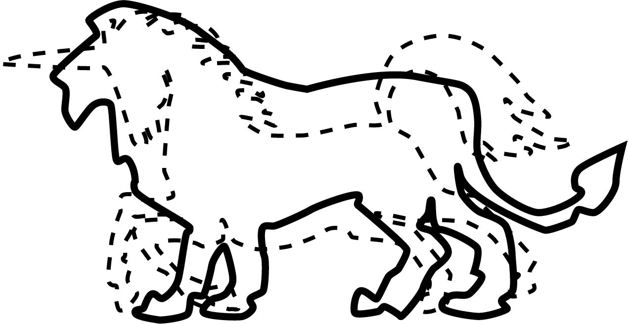
Figure 7.3: Aligned results
First, define a set of the same number of points on each shape. (Lion's point set is P, Unicorn's point set is Q.)
At this time, note that those with the same subscript are in the geometrically corresponding positions as shown in Fig. 7.4 .
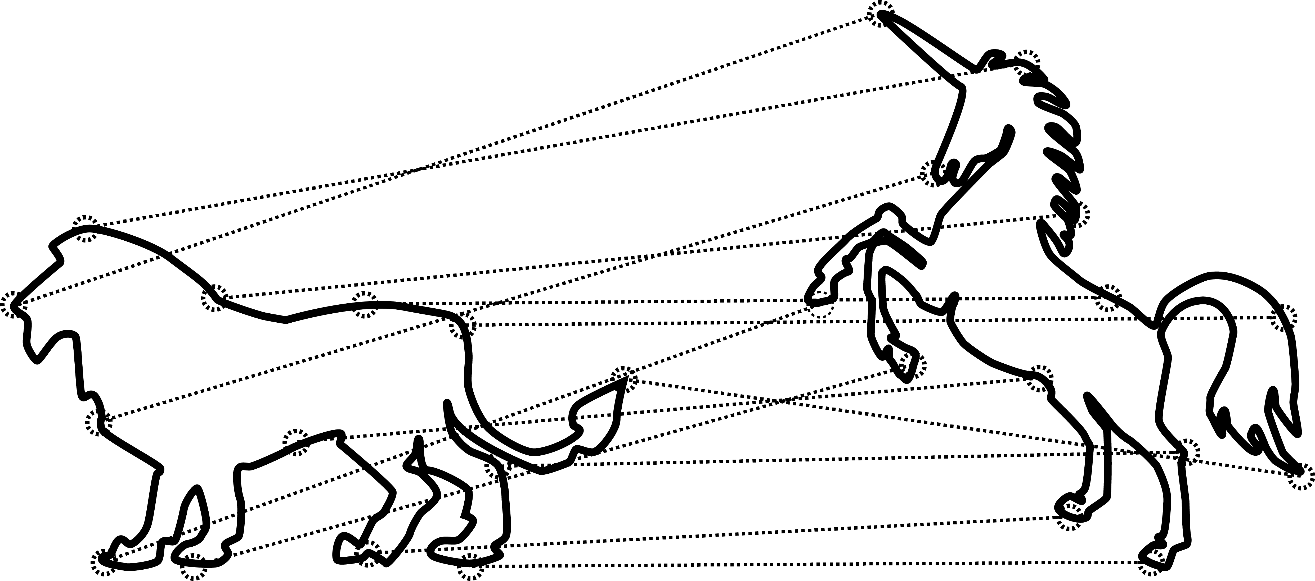
Figure 7.4: Correspondence of point sets
Next, calculate the centroid of each point set.
Assuming that the center of gravity of the unicorn point set is at the same position as the center of gravity of the lion point set, the rotation matrix \ mbox {\ boldmath $ R $} is applied to the unicorn point set, and the vector \ mbox {\ boldmath $ t Since the result of the $} translation is equal to the center of gravity of the lion, the following equation can be derived.
When this is transformed,
And further deformed,
Will be.
Therefore, from this equation, if the rotation matrix \ mbox {\ boldmath $ R $} is obtained, the translation vector \ mbox {\ boldmath $ t $} is automatically obtained. Here, the original point Define a set of points from the position of, minus the center of gravity of each.
This makes it possible to perform calculations with local coordinates with the center of gravity of each point set as the origin.
Next, the variance-covariance matrix \ mbox {\ boldmath of \ mbox {\ boldmath $ p $} _ {i} ^ {\ prime}, \ mbox {\ boldmath $ q $} _ {i} ^ {\ prime} Calculate $ H $} .
This variance-covariance matrix \ mbox {\ boldmath $ H $} stores information such as the variability of the two point sets. Here the product of the vectors \ mbox {\ boldmath $ q $} _ {i } ^ {\ prime} {\ mbox {\ boldmath $ p $} _ {i} ^ {\ prime}} ^ {T} is an operation called direct product (outer product), unlike the normal vector internal product operation. The direct product of the vectors produces a matrix. The direct product of the two-dimensional vectors is defined below.
In addition, the covariance matrix \ mbox {\ boldmath $ H $} is singularly decomposed.
In the result of singular value decomposition, \ mbox {\ boldmath $ \ sum $} is a matrix representing expansion and contraction, so the desired rotation matrix \ mbox {\ boldmath $ R $} is
(The detailed derivation method is a little advanced, so I will omit it here.)
Finally, the translation vector \ mbox {\ boldmath $ t $} can be calculated from the obtained rotation matrix and equation (\ ref {trans}) .
In this implementation, the algorithm in the previous section is just dropped into the code, so detailed explanation is omitted. In addition, all the processing is completed in the Start function in ShapeMaching.cs.
Listing 7.2: ShapeMatching (ShapeMaching.cs)
 1: // Set p, q
 2: p = new Vector2[n];
 3: q = new Vector2[n];
 4: centerP = Vector2.zero;
 5: centerQ = Vector2.zero;
 6:
 7: for(int i = 0; i < n; i++)
 8: {
 9:     Vector2 pos = _destination.transform.GetChild(i).position;
10:     p[i] = pos;
11:     centerP += pos;
12:
13:     pos = _target.transform.GetChild(i).position;
14:     q[i] = pos;
15:     centerQ += pos;
16: }
17: centerP /= n;
18: centerQ /= n;
19:
20: // Calc, p, q!
21: Matrix2x2 H = new Matrix2x2(0, 0, 0, 0);
22: for (int i = 0; i < n; i++)
23: {
24:     p[i] = p[i] - centerP;
25:     q[i] = q[i] - centerQ;
26:
27:     H += Matrix2x2.OuterProduct(q[i], p[i]);
28: }
29:
30: Matrix2x2 u = new Matrix2x2();
31: Matrix2x2 s = new Matrix2x2();
32: Matrix2x2 v = new Matrix2x2();
33: H.SVD(ref u, ref s, ref v);
34:
35: R = v * u.Transpose();
36: Debug.Log(Mathf.Rad2Deg * Mathf.Acos(R.m00));
37: t = centerP - R * centerQ;
I was able to safely align the shape of the unicorn with the shape of the lion.
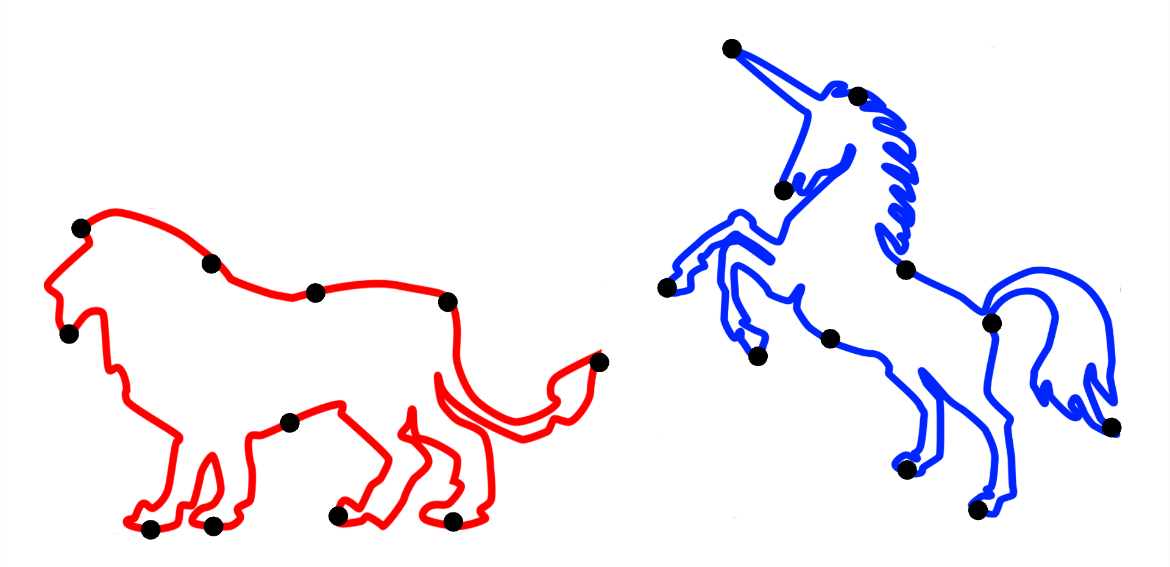
Figure 7.5: Before execution
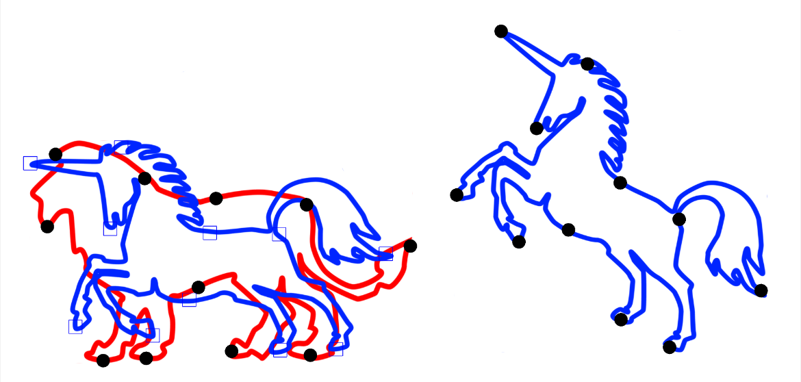
Figure 7.6: After execution
In this section, we explained the implementation of the Shape Matching method using singular value decomposition. This time, it was implemented in 2D, but it can also be implemented in 3D with the same algorithm. I think that there were many, but I hope that you will take this opportunity to become interested in the application method of matrix arithmetic in the CG field and deepen your learning.